Homework 5
Due Nov 13 on canvas
1
The tips data in the reshape package contains a dataset of tips recorded by a waiter. Take a look at the histograms produced by the code below and notice the two tippers with unusually high tip percentages.
library(ggplot2)
library(reshape2)
library(coin) # you might need to install this one if you haven't already
tips$percent <- with(tips, tip/total_bill * 100)
qplot(percent, data = tips) + facet_wrap(~ sex, ncol = 1)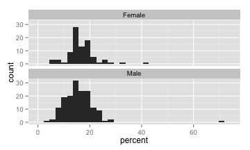
The following code, runs a two sample t-test and a wilcoxon rank sum test to compare male to female tippers, both with and without the two tippers with unusually high tip percentages.
library(reshape2)
library(coin) # you might need to install this one if you haven't already
tips$percent <- with(tips, tip/total_bill * 100)

t.test(percent ~ sex, data = tips, var.equal = TRUE) # with outliers
t.test(percent ~ sex, data = subset(tips, percent < 40), var.equal = TRUE) # without outliers
wilcox_test(percent ~ sex, data = tips, conf.int = TRUE)  # with outliers
wilcox_test(percent ~ sex, data = subset(tips, percent < 40), conf.int = TRUE) # without outliers
For each test, compare the p-values and confidence intervals based on the data with and without the outlier. Based on your comparisons, does the Wilcoxon Rank Sum appear more resistent to outliers than the two sample t-test? Justify your answer.
2
The PlantGrowth dataset contains the dried weight of plants in a randomized experiment comparing two treatment conditions to a control.
head(PlantGrowth)## weight group
## 1 4.17 ctrl
## 2 5.58 ctrl
## 3 5.18 ctrl
## 4 6.11 ctrl
## 5 4.50 ctrl
## 6 4.61 ctrl-
Produce a plot of the data to compare the plant weights for the three conditions (control, treamtment 1 and treatment 2).
-
Produce summary statistics of the weights (average, sd, and sample size) for the three conditions.
-
Find the pooled standard deviation of weight and it’s degrees of freedom.
-
Find the residual sum of squares for the full model (a different mean weight for each condition) and the reduced model (a single mean weight for each condition). Hint: see the code posted for the Nov 4 lecture.
-
(a) Verify that the residual sum of squares for the full model is the pooled standard deviation squared, multiplied by it’s degrees of freedom.
(b) Verify that the residual sum of squares for the reduced model is the squared standard deviation of all the weights (treated as being in one group, i.e.
sd(PlantGrowth$weight)^2) multiplied by n-1. -
The sums of squares from part 4, are items 1 and 2 in Display 5.10 (in Sleuth and the lecture slides). Using Display 5.10 as a guide, fill in the rest of the ANOVA table by hand. (You can use R:
1 - pf(f.stat, df1, df2)to get the p-value). You can copy, paste and edit this table template to include your result in your R file:#' #' #' Source of variation | Sum Sq | Df | Mean Sq | F statistic | p-value #' --------------------- | ----------- | ---- | --------- | ------------- | ---------- #' **Between groups** | 1927.08 | 6 | 321.2 | 6.718 | 6.096e-05 #' **Within groups** | 1864.45 | 39 | 47.81 | | #' **Total** | 3791.53 | 45 | | | #' #' Table: Analysis of Variance Table #' -
Summarise the results of the F-test in a statistical summary (one sentence).
-
Find a 95% confidence interval for the treament effect of treatment 1 compared to the control, and report the result in a sentence.