Labs are designed to be self-paced. If you get stuck, ask a neighbor first. If you can’t solve the problem your TA is there to help! Discuss the questions in bold with your neighbor too.

Goals

• Writing a script from scratch
• Learn about the basic data object in R the data.frame
• Learn some basic data summary code
• Make your first R plot

Getting started

Open RStudio. Copy and paste this code into the console and hit Enter, to get the packages that contain the Sleuth datasets and the OpenIntro datasets.

install.packages(c("Sleuth3", "openintro"))

Instead of starting with a notebook I’ve written, today you will write your own. This is how I generally work:

1. Open a new R script file
2. Write R code in the file (and run it as I go with “Run” (not “Compile”!))
3. Once I’m satisfied I’ve done all the computation I need I add comments and Compile.
4. Save both the .R and .docx files.

So, let’s follow that procedure as we learn about R.

Open your ST411/511 project in RStudio (this might be a good time to make sure this is in ONID).

Open a new R script file (File -> New -> R Script). Save it as lab1.R (File -> Save).

Copy and paste the following into your script. Highlight the three lines and hit Run (the button, or Ctrl + Enter (win) or Cmd + Enter (mac)).

library(ggplot2)
library(Sleuth3)
library(openintro)

This loads three packages: ggplot2, Sleuth3 and OpenIntro. You’ll always need these three lines at the start of your script if you plan on using data from the book, or plotting using ggplot2.

Data in R

The basic object for storing data in R is the data.frame. Dataframes are just like tables, they are rectangular with rows and columns. Usually we put observations in the rows and variables in the columns, so that each row represents an observational unit.

We will mostly be using data straight from the Sleuth3 package. To see a list of the data in this package, copy and paste this into the Console:

data(package = "Sleuth3")

To look at one of the datasets just type it’s name in the Console

case0101

The console will display the entire dataset, here we can see there are two columns named Score and Treatment. You can find out more about the dataset by using the question mark (?) in the Console

?case0101

This will open some help in the “Help” window. What do the two columns Score and Treatment represent?

In general you can use the ? to get help on data or functions. Try in the Console:

?mean

Other useful functions for exploring a data.frame are str, head and summary. Copy and paste the following lines into your script.

str(case0101)
head(case0101)
summary(case0101)

Highlight them and run them. What do each of those functions do? Remember you can use ? if you can’t figure it out.

Basic data summaries

We’ve been talking a lot in lecture about sample averages and sample standard deviations, but we haven’t calculated any in R yet. Let’s practice with a dataset from openintro called textbooks. In the console scan the help for the dataset and have a look at the data:

?textbooks
textbooks

Sound familiar? There’s a column called diff that contains the difference in price between textbooks at amazon and the UCLA bookstore. Let’s find the sample average and sample sd of these differences. In the console type

textbooks$diff

textbooks$diff tells R we want the column called diff from the data.frame called textbooks (more on this another day). You should see a list of numbers, these are our sample of differences in price.

In your script copy the following lines and run them:

mean(textbooks$diff) # x bar
sd(textbooks$diff)   # s
length(textbooks$diff) # n

Let’s say we want a one-sample t 95% confidence interval for the population mean difference in price. The above code printed out what we need, but let’s save them instead so we can reuse them. Edit the code in your script to read, then run it:

xbar <- mean(textbooks$diff) # x bar
s <- sd(textbooks$diff)   # s
n <- length(textbooks$diff) # n

The <- says save the output from the code on the right into an object given by the name of the left. You can see their values in the Workspace window, or by typing their names in the console.

Ok, now a 95% confidence one sample t interval is,

se_xbar <- s/sqrt(n)
df <- n-1
xbar - qt(0.975, df) * se_xbar
xbar + qt(0.975, df) * se_xbar

Can you relate that code back to the formulas in the lecture slides? Any new functions there?

Ok, so far you should just have R code in your R script file. Try Compiling it. Your output should just be R code and R output. You might want to add some comments now. In your R script add the following line:

#'  With 95% confidence the price of a textbook is on average between $9.44 and $16.09 cheaper at Amazon than at the UCLA bookstore.

Compile again.

Optional

We ended up looking for the confidence interval in our output, then rounding and writing it out by hand. You can also make R do the work for you. Try adding the following to your notebook.

lwr <- xbar - qt(0.975, df) * se_xbar
upr <- xbar + qt(0.975, df) * se_xbar
#'  With 95% confidence the price of a textbook is on average between $`r round(lwr,2)`  and $`r round(upr,2)` cheaper at Amazon than at the UCLA bookstore.

Note how we save the upper and lower ends of the interval and then refer to them in our text. Compile and see how the R code in the text is converted to output.

End Optional

A simple plot

We will be using the ggplot2 package to do all of our plots, and we will learn more about it in lecture this week. The primary function we will use is qplot. Copy and paste the following into your R script, then run it:

qplot(Treatment, Score, data = case0101)

Repeat with the following plotting commands.

qplot(Treatment, Score, data = case0101, 
      geom = "boxplot")
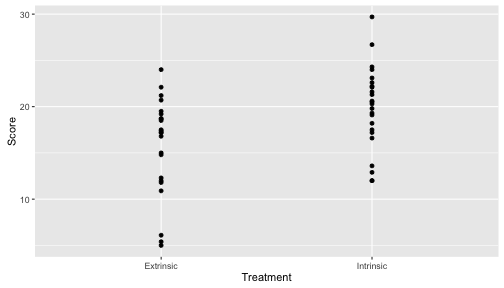
qplot(Treatment, Score, data = case0101, 
      geom = "violin")
qplot(Treatment, Score, data = case0101) +
  geom_dotplot(binaxis = "y", 
               stackdir = "center")

What’s changing in each of these plots and what stays the same? Can your relate the changes in the plots to the changes in the code?

Save your script. If you still have time, try the following challenge. Otherwise, close RStuido and log off. You can also look at an example of how your script should look here: lab-1-example.r

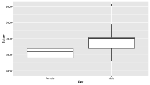
Plot Challenge

If you have time, try to reproduce this plot (using the case0102 data)?: