Today’s lab is a little different to last week, in that I will give you very little code. Try to recall from memory before looking Friday’s slides to remind yourself of the appropriate commands. You probably want to keep all your code in an R script and run your commands from there (no need to “Compile” today).

Goals

• Practice subsetting data frames to get observations of interest.
• Practice plotting data to examine their distribution

Subsetting

In lecture Friday we discussed three types of subsetting: using $ to get a column from a data.frame, using subset to return certain rows of a data.frame, and very briefly using [ to get more general subsets. Today in lab we will practice the first two.

This section is adapted from the OpenIntro labs (http://www.openintro.org/) and is released under a Creative Commons BY-NC-SA 3.0 license.

The Behavioral Risk Factor Surveillance System (BRFSS) is an annual telephone survey of 350,000 people in the United States. As its name implies, the BRFSS is designed to identify risk factors in the adult population and report emerging health trends. For example, respondents are asked about their diet and weekly physical activity, their HIV/AIDS status, possible tobacco use, and even their level of healthcare coverage. The BRFSS Web site (http://www.cdc.gov/brfss) contains a complete description of the survey, including the research questions that motivate the study and many interesting results derived from the data. We will focus on a random sample of 20,000 people from the BRFSS survey conducted in 2000. While there are over 200 variables in this data set, we will work with a small subset.

We begin by loading the data set of 20,000 observations into the R workspace. After launching RStudio, enter the following command,

load(url("http://stat511.cwick.co.nz/data/cdc.rda"))

This loads a data.frame of the data, cdc. With 20,000 observations you do not want to simply view the whole data.frame. Try head or one of the other commands (can you remember any more?) we have learnt to take a peak at the data. The function names just returns the column names in a data.frame, for example:

names(cdc)

This returns the names genhlth, exerany, hlthplan, smoke100, height, weight, wtdesire, age, and gender. Each one of these variables corresponds to a question that was asked in the survey. For example, for genhlth, respondents were asked to evaluate their general health, responding either excellent, very good, good, fair or poor. The exerany variable indicates whether the respondent exercised in the past month (1) or did not (0). Likewise, hlthplan indicates whether the respondent had some form of health coverage (1) or did not (0). The smoke100 variable indicates whether the respondent had smoked at least 100 cigarettes in her lifetime. The other variables record the respondent’s height in inches, weight in pounds as well as their desired weight, wtdesire, age in years, and gender.

Say, we are interested in the average age of the male respondents. First, we would subset out the male respondents. To do that we need to know which rows correspond to males. A good guess would be that the gender column can tell us, and a quick look

summary(cdc$gender)

suggests males are denoted with m. So, we can create a new data.frame with just the males,

males <- subset(cdc, gender == 'm')
head(males)

Now we can take the average of the age column

mean(males$age)

Your answer might differ due to different rounding conventions.

Following the same steps answer the following questions:

1. What is the average age of female respondents?

2. Find the median weight of respondents without health insurance. (Hint: create a new data.frame of people without health insurance, then find the median of the weight column in that new data.frame. There is a median function.)
3. Find the median weight of respondents without health insurance and who had not exercised in the last month.

4. How many females are younger than age 30?

5. (Harder) Find the average difference between weight and wtdesire (the desired weight) for all respondents and for males and females separately.

If you are interested in more general subsetting with the [, check out the rcookbook.

More plotting practice

Try to recreate the following plots:

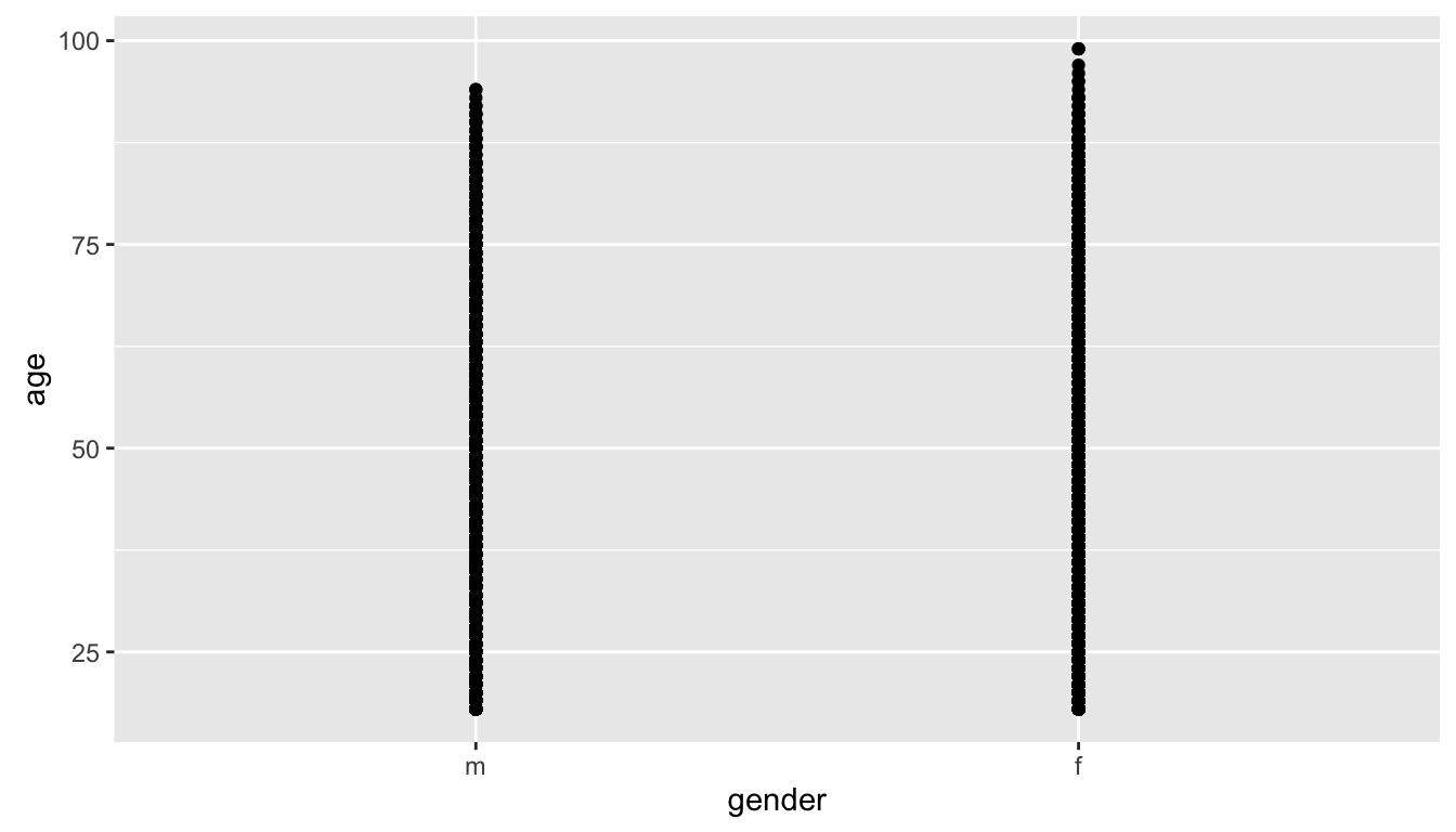
1. Dotplots of age by gender. Note how useless this plot is.
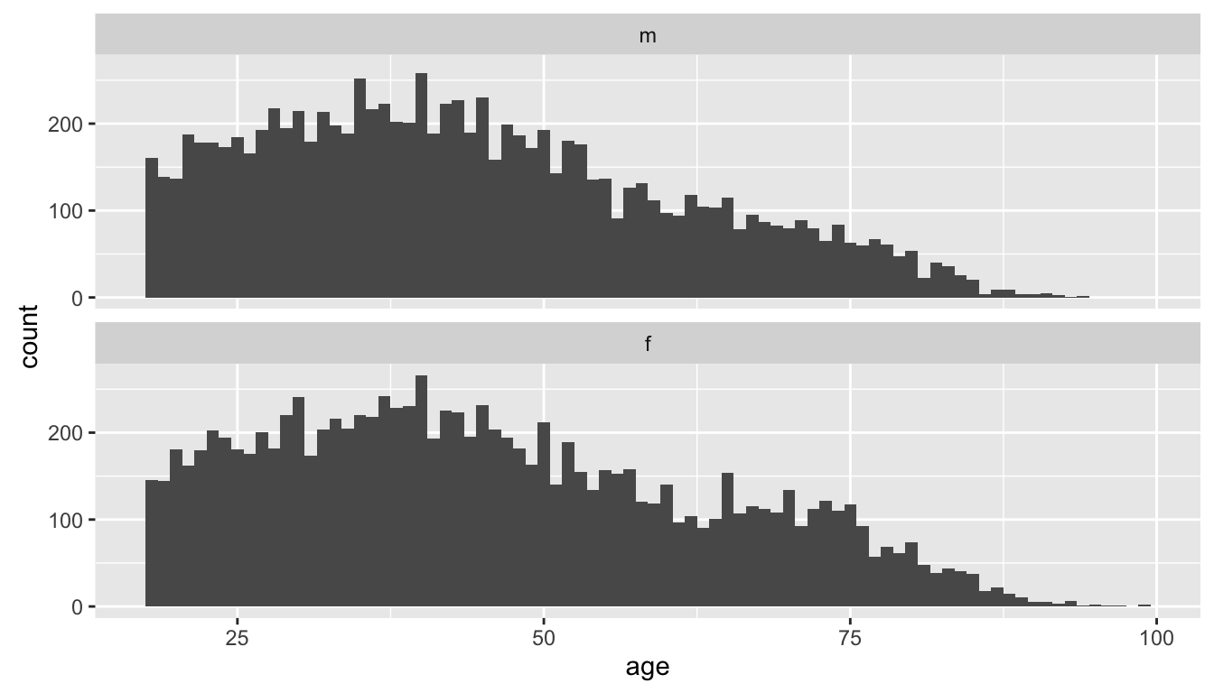
2. Histograms of age by gender. Much more useful.
3. Boxplots of weight by whether respondents had exercised in the last month. Hint: the exerany, variable is stored as a number, but we want to use it like a category, wrap it in factor, i.e. factor(exerany) to make R interpret it as a category.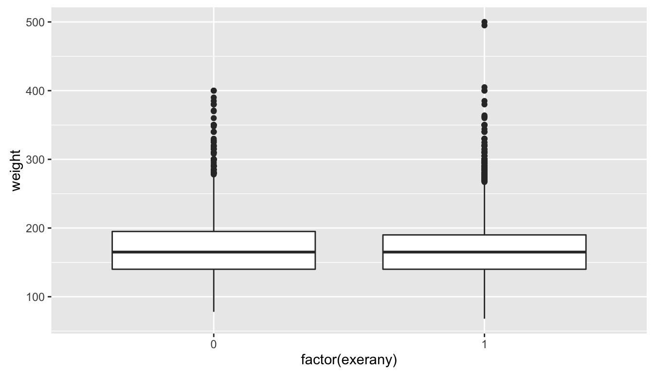
4. Boxplots of weight by gender, coloured by gender. Hint: add a colour = gender argument to the qplot command.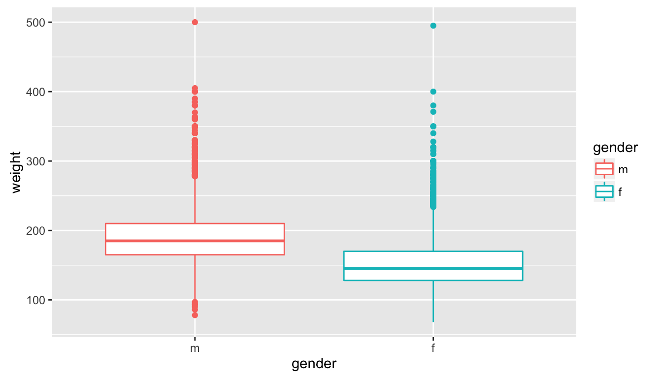
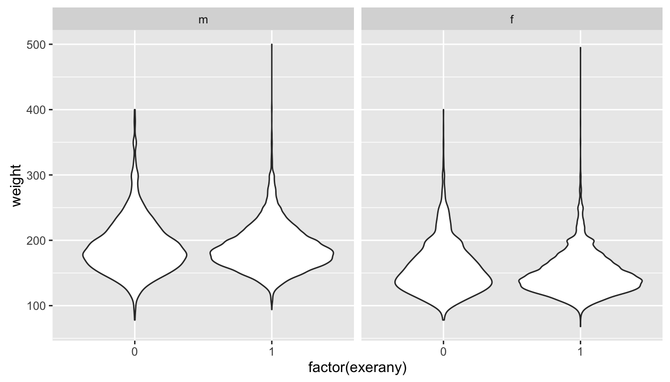
5. Violin plots of weight by whether respondents had exercised in the last month faceted by gender.
6. Come up with your own question on interest about the cdc data and answer it using a plot.
7. Try adding ` + theme_bw()` to any of your previous plots
8. Try adding ` + ggtitle(“Hello, I’m a title”)` to any of your previous plots