Goals

• Vectors in R and an example of a two group comparison when there are multiple groups.
• Gain some intuition on the ratio of the sum of squares in an F-test.
• Code for the two group tests we have seen for your reference (optional)

Two group comparisons when there are multiple groups

For today’s lab we’ll use a subset of an experiment that examined the length of teeth in each of 10 guinea pigs at each of three dose levels of Vitamin C (0.5, 1, and 2 mg) delivered through orange juice.

library(ggplot2)
tooth <- subset(ToothGrowth, supp == "OJ")
qplot(factor(dose), len, data = tooth)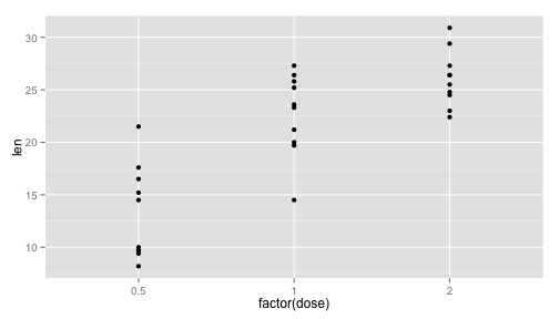

In class I demonstrated how you could get the average, standard deviation and sample size within each group.

avgs <- with(tooth, tapply(len, dose, mean))
avgs
sds <- with(tooth, tapply(len, dose, sd))
sds
ns <- with(tooth, tapply(len, dose, length))
ns

These three objects, avgs, sds and ns are vectors. It’s useful at this point to learn a little more about manipulating vectors. Square brackets, [, are used to subset vectors. You can use a number, i.e.,

avgs[2]

pulls out the 2nd value or you can use a name, i.e.,

avgs["0.5"]

pulls out the entry with the column name “0.5”. Here things are a little confusing because our column names are numbers. These two commands mean different things:

avgs[1]      # give me element number 1
avgs["1"]    # give me the element with name "1"

Math with vectors works like math with numbers but everything happens element by element and the result is a vector. For example,

avgs + 10     # add ten to each number
avgs^2        # square each number
sqrt(ns)      # squareroot each number

If two vectors have the same length, you can do math on them one entry at a time. For example,

sds / sqrt(ns)   

takes each standard deviation and divides it by the sqrt of the number of subjects in that group.

If two vectors don’t have the same length, R repeats the shorter one until it is the same length and warns you (you shouldn’t ever need to do this in this class),

x <- c(1, 10) # a new vector of length 2
x
ns + x

## Warning in ns + x: longer object length is not a multiple of shorter
## object length

There are also functions that are specially designed to work with vectors, some of which we have already seen

sum(ns)     # add all the numbers in the vector up (the total sample size, n)  
prod(ns)    # multiply all the numbers in the vector together
length(ns)  # how long is this vector?

Can you pull apart the command to calculate the pooled standard deviation and understand what is happening?

sp <- sqrt(sum((ns - 1) * sds ^ 2) / sum(ns - 1))
sp

Let’s calculate a 95% confidence interval for the treatment effect on tooth length of the dose of 1 compared to the dose of 0.5. The usual two-sample t-test procedure can be used, with the pooled standard deviation based on all the groups and the corresponding degrees of freedom. It’s always safer to refer to the entries by name rather than number.

est <- avgs["0.5"] - avgs["1"]   # the difference in sample averages (0.5 dose - 1 dose)
se <- sp * sqrt( 1/ns["0.5"] + 1/ns["1"])   # the s.e.
df <- sum(ns) - length(ns)

est + c(-1, 1) * qt(0.975, df) * se

With 95% confidence we estimate that the dose of 1 milligrams increases the tooth length by between 6.0 and 12.9 units compared to the 0.5 milligram dose.

Note that subsetting to just the groups of interest and using t.test does not give the same answer:

t.test(len ~ dose, data = subset(tooth, dose %in% c(0.5, 1)),
  var.equal = TRUE)

This approach throws away the information the third group gives us about the common population standard deviation and is inefficient. Don’t do this in HW #5

Understanding the sums of squares in the F-test

I’ve created a little interactive example of the sum of squares in an F-test. Go to: https://cwickham.shinyapps.io/anova/

A web browser should pop up with some sliders and plots.

The first plot shows three population distributions. Their means and common standard deviation are controllable with the sliders. Change them and watch the distributions change.

Click the button “Take samples” to simulate taking samples from these three population distributions. The other four plots will update.

The dotplot shows a plot of the sampled data, along with the overall sample average (the grey line) and the group averages (coloured lines).

The next plot shows the histogram of the residuals from the separate means model (full model) and visually displays the variation within groups. By definition these residuals will always be less spread out than those from the equal means model. The “Within group sum of squares” is the sum of the square of these residuals. Again, you can think of the Within group sum of squares divided by the within group d.f. (MSS within) as an estimate of the variance of this distribution.

The fourth plot shows the distribution of the deviation of the group averages from overall sample average and visually displays the variation between groups. These deviations sum and squared give the “Between group sum of squares”. Again, you can think of the Between group sum of squares divided by the between group d.f. (MSS between) as an estimate of the variance of this distribution.

The F-statistic is the ratio of between to within mean sum of squares. You can think of this as a ratio of the variance of the group averages and the variance within groups. A large F-statistic says the spread of the group averages is much larger than the spread we would normally see within a group, and gives us evidence that not all the groups have the same mean.

Ok, now it’s time for you to experiment with changing some of the variables involved.

Try setting all of the means to the same number (the equal means model). How does the spread within groups compare to between groups?

Try making the standard deviation smaller (or larger). How does the within group variation change, and how does the between group variation change?

Code for the two group tests

You should know how to get the Wilcoxon Rank Sum and Sign test statistics by hand (for very small datasets) but in practice it is more useful for you to have R do them for you.

Two independent groups

There are some commonalities in most of the functions to do the tests. They all take a special R object called a formula of the form Response ~ Groups. We read this as “Response is modelled by Groups”. R estimates a different mean Response in each level of the Groups variable, and tests if they are different. “Response” and “Groups” should be the columns in the appropriate data.frame that contain the response and the grouping variable. All the functions also take a data argument to specify the data.frame in which the Response and Groups columns are stored.

Remember the Creativity dataset,

library(Sleuth3)
head(case0101)

We wanted to test for a difference in mean Score for each group in Treatment. This is an example of a “two independent samples” comparison. Our formula would be Score ~ Treatment and we would also specify the data.frame with data = case0101.

The four test’s we have covered for this comparision are: the randomization test using sample averages, the two-sample t-test, the Wilcoxon rank sum, and Welch’s two sample t-test.

library(coin)
# Randomization test
oneway_test(Score ~ Treatment, data = case0101, distribution = "approximate")
# Two sample t-test
t.test(Score ~ Treatment, data = case0101, var.equal = TRUE)
# Wilcoxon rank sum test
wilcox_test(Score ~ Treatment, data = case0101, conf.int = TRUE)
# Welch's t-test
t.test(Score ~ Treatment, data = case0101)

Notice how the first two arguments are always the same. Also note the results from all of these tests are pretty close. Since, the creativity data looks to satisfy both the Normality and equal population standard deviations assumptions, and there aren’t any outliers, all of these tests would be appropriate.

One sample or two paired groups

Recall the Schizophrenia dataset,

head(case0202)

We have seen three tests for paired data: the paired t-test, sign test and Wilcoxon Signed Rank test. The procedures aren’t quite as consistent for paired data. The t-test function requires the differences, the sign test we do almost by hand and the Wilcoxon signed rank test uses the formula idea in a different way,

# first find the differences
diffs <- with(case0202, Unaffected - Affected)

# Paired t-test
t.test(diffs)
# Sign test
binom.test(sum(diffs > 0), sum(diffs != 0))
# Wilcoxon Signed Rank test
wilcoxsign_test(Unaffected ~ Affected, data = case0202, 
            distribution = exact(), zero.method = "Wilcoxon")